%matplotlib inline
import numpy as np
np.set_printoptions(precision=2)
import pandas as pd
import matplotlib.pyplot as plt
import seaborn as snsBreastCancerPredictAI
| Author(s): | Mahbub Alam |
Introduction
Breast Cancer Prediction using Machine Learning:
This project uses the Breast Cancer Wisconsin Diagnostic Dataset to build a machine learning model that can classify tumors as malignant or benign.
It demonstrates an end-to-end ML workflow:
- Data loading & cleaning
- Exploratory data analysis (EDA)
- Preprocessing
- Model training
- Model validation
- Insights and conclusions
Such predictive modeling can support early detection and assist healthcare professionals, though models should never replace medical diagnosis.
Data loading and cleaning
We start by loading the cleaned breast cancer dataset. Each row represents a tumor with various features extracted from digitized images of a fine needle aspirate (FNA). The target column indicates whether the tumor is malignant (cancerous) or benign (non-cancerous).
Machine learning algorithms require clean, numerical, and scaled data. Steps:
- Handle missing values (if any)
- Find duplicates
- Encode target labels (Malignant = 1, Benign = 0)
- Split dataset into training and testing sets
Looks like there is an extra comma at the end of the columns. This creates an empty column called “Unnamed: 32”. We shall delete it.
df = pd.read_csv('breast_cancer_data.csv')

# print(df.head())
print(df.columns)
print(f"")
print(df.info())

df = df.drop(columns="Unnamed: 32")
print(f"")

# No missing data
missing_data = df.isna().any()
print(f"Missing data? - {'Yes' if missing_data.any() else 'No'}")

# Drop perfect duplicate rows
before = len(df)
df = df.drop_duplicates()
print(f"Duplicates removed: {before - len(df)}")

# saving cleaned data
df.to_csv('breast_cancer_data_cleaned.csv', index=False)

# Data already cleaned, loading clean data
# Not necessary, just to illustrate
df = pd.read_csv('breast_cancer_data_cleaned.csv')
# print(df.columns) # Output: ['id', 'diagnosis', 'radius_mean', 'texture_mean', 'perimeter_mean', 'area_mean', 'smoothness_mean', 'compactness_mean', 'concavity_mean', 'concave points_mean', 'symmetry_mean', 'fractal_dimension_mean', 'radius_se', 'texture_se', 'perimeter_se', 'area_se', 'smoothness_se', 'compactness_se', 'concavity_se', 'concave points_se', 'symmetry_se', 'fractal_dimension_se', 'radius_worst', 'texture_worst', 'perimeter_worst', 'area_worst', 'smoothness_worst', 'compactness_worst', 'concavity_worst', 'concave points_worst', 'symmetry_worst', 'fractal_dimension_worst']
Index(['id', 'diagnosis', 'radius_mean', 'texture_mean', 'perimeter_mean',
'area_mean', 'smoothness_mean', 'compactness_mean', 'concavity_mean',
'concave_points_mean', 'symmetry_mean', 'fractal_dimension_mean',
'radius_se', 'texture_se', 'perimeter_se', 'area_se', 'smoothness_se',
'compactness_se', 'concavity_se', 'concave_points_se', 'symmetry_se',
'fractal_dimension_se', 'radius_worst', 'texture_worst',
'perimeter_worst', 'area_worst', 'smoothness_worst',
'compactness_worst', 'concavity_worst', 'concave_points_worst',
'symmetry_worst', 'fractal_dimension_worst', 'Unnamed: 32'],
dtype='object')
<class 'pandas.core.frame.DataFrame'>
RangeIndex: 569 entries, 0 to 568
Data columns (total 33 columns):
# Column Non-Null Count Dtype
--- ------ -------------- -----
0 id 569 non-null int64
1 diagnosis 569 non-null object
2 radius_mean 569 non-null float64
3 texture_mean 569 non-null float64
4 perimeter_mean 569 non-null float64
5 area_mean 569 non-null float64
6 smoothness_mean 569 non-null float64
7 compactness_mean 569 non-null float64
8 concavity_mean 569 non-null float64
9 concave_points_mean 569 non-null float64
10 symmetry_mean 569 non-null float64
11 fractal_dimension_mean 569 non-null float64
12 radius_se 569 non-null float64
13 texture_se 569 non-null float64
14 perimeter_se 569 non-null float64
15 area_se 569 non-null float64
16 smoothness_se 569 non-null float64
17 compactness_se 569 non-null float64
18 concavity_se 569 non-null float64
19 concave_points_se 569 non-null float64
20 symmetry_se 569 non-null float64
21 fractal_dimension_se 569 non-null float64
22 radius_worst 569 non-null float64
23 texture_worst 569 non-null float64
24 perimeter_worst 569 non-null float64
25 area_worst 569 non-null float64
26 smoothness_worst 569 non-null float64
27 compactness_worst 569 non-null float64
28 concavity_worst 569 non-null float64
29 concave_points_worst 569 non-null float64
30 symmetry_worst 569 non-null float64
31 fractal_dimension_worst 569 non-null float64
32 Unnamed: 32 0 non-null float64
dtypes: float64(31), int64(1), object(1)
memory usage: 146.8+ KB
None
Missing data? - No
Duplicates removed: 0Exploratory data analysis (EDA)
Understanding the dataset is key before building models. We will:
- Check class distribution (malignant vs. benign)
- Visualize feature distributions
- Explore correlations between features
Class distribution
# Proportion of benign and malignant tumors

print(df['diagnosis'].value_counts())

X = df.drop(columns=["diagnosis", "id"])
y = (df["diagnosis"] == "M").astype("int")
diagnosis
B 357
M 212
Name: count, dtype: int64Visualization
Radius, texture and perimeter – mean, standard error and worst value.
df_benign = df[df["diagnosis"] == "B"]
df_malignant = df[df["diagnosis"] == "M"]

features = X.columns

n_cols = 3
n_rows = 3
size = n_rows * n_cols

fig_name = "Feature Distributions by Diagnosis"
plt.figure(num=fig_name, figsize=(n_rows * 3.5, n_cols * 3.5))

for i in range(size):
    plt.subplot(n_rows, n_cols, i+1)
    feature = features[i//3 + 10 * (i%3)]
    sns.kdeplot(df_benign[feature], color="blue", label="B", fill=False)
    sns.kdeplot(df_malignant[feature], color="magenta", label="M", fill=False)
    plt.legend(loc="upper right", fontsize=8)

plt.suptitle(fig_name, fontsize=14)
plt.tight_layout(pad=2.5, rect=(0, 0.05, 1, 0.95))
plt.subplots_adjust(hspace=0.4, wspace=0.25)

plt.savefig('feature_distribution_eda.jpg')
plt.show()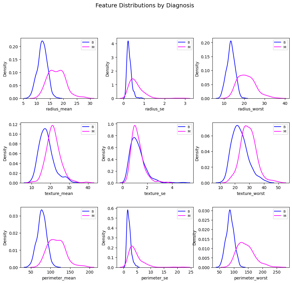
Correlation between features
cols = list(X.columns[:6]) + ["diagnosis"]

fig_name = "Scatter plot of features"
g = sns.pairplot(df[cols],
                 hue="diagnosis",
                 corner=True,
                 plot_kws={'alpha': 0.6, 's': 10, 'edgecolor': 'none'},
                 diag_kind="kde",
                 palette={'B': 'blue', 'M': 'magenta'},
                )

g.fig.set_size_inches(9, 9)
plt.setp(g._legend.get_texts(), fontsize=15)
g._legend.get_title().set_fontsize(15)
g._legend.set_bbox_to_anchor((0.8, 0.7))
g.fig.canvas.manager.set_window_title(fig_name)
g.fig.suptitle(fig_name, fontsize=14, y=0.90)
g.fig.tight_layout(pad=2.5, rect=(0, 0.05, 1, 0.95))
g.fig.subplots_adjust(hspace=0.4, wspace=0.25)

g.fig.savefig('correlation_between_features.jpg')
plt.show()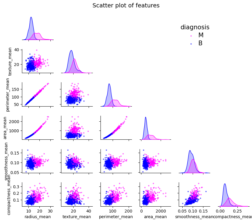
Data Preprocessing
Preprocessing the data with ColumnTransformer and StandardScaler. There are no non-numeric data, we can use StandardScaler safely.
Finally we create train test split for machine learning.
from sklearn.preprocessing import StandardScaler
from sklearn.compose import ColumnTransformer
from sklearn.pipeline import Pipeline

X_features = X.columns

# Only necessary if 2 or more encoders (I am adding just for demo)
pre = ColumnTransformer([
    ('scaler', StandardScaler(), X_features)
])

# # Just for testing. Has to be commmented before model training,
# # since this includes X_test in mean_ and scale_
# X = pd.DataFrame(
#     pre.fit_transform(X),
#     columns=X_features,
#     index=df.index
# )
# print(X.info())

from sklearn.model_selection import train_test_split

X_train, X_test, y_train, y_test = train_test_split(X, y, test_size = 0.2, stratify = y, random_state = 1)
Model Training
We will train multiple classifiers (e.g., Logistic Regression, K Nearest Neighbors, etc.) and Neural Networks and compare their performance to find the most effective model.
Evaluation metrics include:
- Accuracy
- Precision
- Recall
- F1-score
- ROC-AUC
Creating a pipeline of logistic regression
We want to determine the best hyperparameters for LogisticRegression. For this we use GridSearchCV for cross validation. To do this reliably let us use a pipeline.
from sklearn.linear_model import LogisticRegression
from sklearn.model_selection import GridSearchCV, StratifiedKFold

pipe = Pipeline([
    ("pre", pre),
    ('lreg', LogisticRegression(max_iter=10000, solver = 'saga', random_state = 42))
])

hparams = [
    {
        'lreg__penalty' : ['l2', 'l1'],
        'lreg__C' : np.logspace(-3, 3, 13),
        'lreg__class_weight' : [None, 'balanced']
    },
    {
        'lreg__penalty' : ['elasticnet'],
        'lreg__C' : np.logspace(-3, 3, 13),
        'lreg__l1_ratio' : np.linspace(0, 1, 5),
        'lreg__class_weight' : [None, 'balanced']
    }
]

cv = StratifiedKFold(n_splits=5, shuffle = True, random_state = 43)
grid = GridSearchCV(
    pipe,
    hparams,
    scoring = 'average_precision',
    cv=cv,
    n_jobs=4,
    refit=True
)

grid.fit(X_train, y_train)
best_model = grid.best_estimator_

best_model.fit(X_train, y_train)
Pipeline(steps=[('pre',
ColumnTransformer(transformers=[('scaler', StandardScaler(),
Index(['radius_mean', 'texture_mean', 'perimeter_mean', 'area_mean',
'smoothness_mean', 'compactness_mean', 'concavity_mean',
'concave_points_mean', 'symmetry_mean', 'fractal_dimension_mean',
'radius_se', 'texture_se', 'perimeter_se', 'area_se', 'smoothness_se',
'compactness_se', 'co...
'perimeter_worst', 'area_worst', 'smoothness_worst',
'compactness_worst', 'concavity_worst', 'concave_points_worst',
'symmetry_worst', 'fractal_dimension_worst'],
dtype='object'))])),
('lreg',
LogisticRegression(C=np.float64(0.31622776601683794),
class_weight='balanced',
l1_ratio=np.float64(0.25), max_iter=10000,
penalty='elasticnet', random_state=42,
solver='saga'))])In a Jupyter environment, please rerun this cell to show the HTML representation or trust the notebook. On GitHub, the HTML representation is unable to render, please try loading this page with nbviewer.org.
Parameters
| steps | [('pre', ...), ('lreg', ...)] | |
| transform_input | None | |
| memory | None | |
| verbose | False |
Parameters
| transformers | [('scaler', ...)] | |
| remainder | 'drop' | |
| sparse_threshold | 0.3 | |
| n_jobs | None | |
| transformer_weights | None | |
| verbose | False | |
| verbose_feature_names_out | True | |
| force_int_remainder_cols | 'deprecated' |
Index(['radius_mean', 'texture_mean', 'perimeter_mean', 'area_mean',
       'smoothness_mean', 'compactness_mean', 'concavity_mean',
       'concave_points_mean', 'symmetry_mean', 'fractal_dimension_mean',
       'radius_se', 'texture_se', 'perimeter_se', 'area_se', 'smoothness_se',
       'compactness_se', 'concavity_se', 'concave_points_se', 'symmetry_se',
       'fractal_dimension_se', 'radius_worst', 'texture_worst',
       'perimeter_worst', 'area_worst', 'smoothness_worst',
       'compactness_worst', 'concavity_worst', 'concave_points_worst',
       'symmetry_worst', 'fractal_dimension_worst'],
dtype='object')Parameters
| copy | True | |
| with_mean | True | |
| with_std | True |
Parameters
| penalty | 'elasticnet' | |
| dual | False | |
| tol | 0.0001 | |
| C | np.float64(0....2776601683794) | |
| fit_intercept | True | |
| intercept_scaling | 1 | |
| class_weight | 'balanced' | |
| random_state | 42 | |
| solver | 'saga' | |
| max_iter | 10000 | |
| multi_class | 'deprecated' | |
| verbose | 0 | |
| warm_start | False | |
| n_jobs | None | |
| l1_ratio | np.float64(0.25) |
Deciding a threshold for positive results
Given the model (best_model) will give us probabilities for malignant tumor (between 0 and 1). It might seem natural to choose 0.5 as a threshold for positive result, i.e., we might naively want to call a result positive if probability for positive is >= 0.5.
But a serious diagnosis such as breast cancer should have low threshold to avoid high number of false negatives. We want to be absolutely sure that a negative result by the model is truely negative. Also since the ML algorithms output will be reviewed by professional it is prudent to keep the threshold low.
In other words we want our model to have high recall.
To get some ideas about the threshold, below we check the precision recall curve on the test set.
Definitions
P = (actual) positive data points
N = (actual) negative data points
TP = True positive : a data point marked positive by the model that is actually positive
FP = False positive : a data point marked positive by the model that is actually negative
FN = False negative : a data point marked negative by the model that is actually positive
Precision = TP / (TP + FP) : Of the points the model called positive, how many were truly positive? Here TP + FP are the number of data points the model marked positive.
Recall = TP / (TP + FN) : Of the actually positive points, how many did the model correctly find? Here TP + FN are the number of data points that are actually positive.
y_probs = best_model.predict_proba(X_test)[:, 1]

from sklearn.metrics import precision_recall_curve
precision, recall, thresholds = precision_recall_curve(y_test, y_probs)

plt.plot(thresholds, precision[:-1], label="Precision")
plt.plot(thresholds, recall[:-1], label="Recall")
plt.xlabel("Threshold")
plt.ylabel("Score")
plt.title("Precision and recall vs threshold")
plt.legend()
plt.show()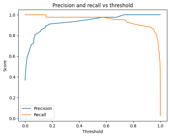
Choosing a threshold
Since this is a medical application, we don’t want the model to miss positives. We care about high recall, about 99%. Let’s find a threshold that achieves this. But we shouldn’t use the test set for choosing this threshold. This might lead to overfitting to the test set.
Let’s use cross validation (CV) again for doing this. More precisely, CV splits the train data (X_train) into CV_train, CV_validation (with different random state than before). We train our best_model on CV_train. On CV_validation the model gives probabilities for positive results.
Now, there are two ways to proceed:
We compare this CV_validation probabilities to relevant y_train to find a threshold for 99% recall. We can take a median of all these thresholds found from the CV splits.
We can take all these probabilities and stack them to get an array, (the same as y_test) which we compare to y_test to get a threshold for 99% recall.
The second method is more robust for medical applications, it collects validation signal on the whole training set (each point predicted by a model that didn’t see it).
def pick_threshold_for_recall(y_true, y_probs, target_recall=0.99):
    """
    Returns the highest threshold whose recall >= target_recall.
    Using the highest such threshold usually gives better precision.
    """
    _, recall, thresholds = precision_recall_curve(y_true, y_probs)
    # precision/recall have length = len(thresholds)+1; align by dropping the first PR point
    recall_t = recall[:-1]
    thresholds_t = thresholds

    # indices where recall constraint is satisfied
    ok = np.where(recall_t >= target_recall)[0]
    if len(ok) == 0:
        # cannot reach target recall; fall back to threshold=0 (max recall)
        chosen = 0.0
    else:
        # choose the largest threshold that still satisfies recall >= target
        chosen = thresholds_t[ok[-1]]
    return float(chosen)

from sklearn.base import clone

cv_thresh = StratifiedKFold(n_splits=5, shuffle=True, random_state=123)  # NEW seed
oof_probs = np.empty(len(y_train), dtype=float) # Out of fold probs

for tr, va in cv_thresh.split(X_train, y_train):
    # start the best_model with initial state
    est = clone(best_model)
    est.fit(X_train.iloc[tr], y_train.iloc[tr])
    oof_probs[va] = est.predict_proba(X_train.iloc[va])[:, 1]

# pick threshold on OOF to hit target recall
threshold = pick_threshold_for_recall(y_train, oof_probs, target_recall=0.99)
Saving the model and the threshold
At this point we can save the model and the threshold for future use.
import joblib

# final refit on full train, then apply fixed threshold on test
best_model.fit(X_train, y_train)

# save to file
joblib.dump(best_model, "best_model.pkl")

import json
with open("chosen_threshold.json", "w") as f:
    json.dump({"threshold": float(threshold)}, f)

# # Only when loading saved model and threshold
# # load best_model from file
# best_model = joblib.load("best_model.pkl")

# # load back
# with open("chosen_threshold.json") as f:
#     threshold = json.load(f)["threshold"]
Model Evaluation
We compare model performance on the test set. Metrics and confusion matrices help us assess:
- How well the model detects malignant tumors (sensitivity/recall)
- How well it avoids false positives (specificity/precision)
The ROC curve and AUC score further summarize predictive power.
y_preds = (y_probs >= threshold).astype(int)

from sklearn.metrics import precision_recall_curve
precision, recall, thresholds = precision_recall_curve(y_test, y_probs)

plt.plot(thresholds, precision[:-1], label="Precision")
plt.plot(thresholds, recall[:-1], label="Recall")
plt.axvline(x=threshold, color="red", linestyle="--", linewidth=1.5,
            label=f"Chosen threshold = {threshold:.3f}")
plt.text(threshold*1.2, 0.5, f"{threshold:.3f}", rotation=90,
         va='center', ha='right', color='red', fontsize=9)
plt.xlabel("Threshold")
plt.ylabel("Score")
plt.title("Precision and recall vs threshold")
plt.legend()
plt.show()

# from sklearn.metrics import PrecisionRecallDisplay
# _ = PrecisionRecallDisplay(precision=precision, recall=recall).plot()
# plt.show()

from sklearn.metrics import accuracy_score, precision_score, recall_score, confusion_matrix

def metrics_at_threshold(y_true, y_preds, threshold):
    return {
        "threshold": threshold,
        "precision": precision_score(y_true, y_preds, zero_division=0),
        "recall": recall_score(y_true, y_preds, zero_division=0),
        "accuracy": accuracy_score(y_true, y_preds),
        "confusion_matrix": confusion_matrix(y_true, y_preds)  # [[TN, FP],[FN, TP]]
    }


report = metrics_at_threshold(y_test, y_preds, threshold)

# results
print("\nModel report:")
for metric, value in report.items():
    if metric == "confusion_matrix":
        print(f"    {metric:20} :")
        print(f"{value}")
    else:
        print(f"    {metric:20} : {value:.4f}")


# Output:
# {'threshold': 0.18020206682554823, 'precision': 0.9111111111111111, 'recall': 0.9761904761904762, 'accuracy': 0.956140350877193,
#  'confusion_matrix': array([[68,  4],
#        [ 1, 41]])}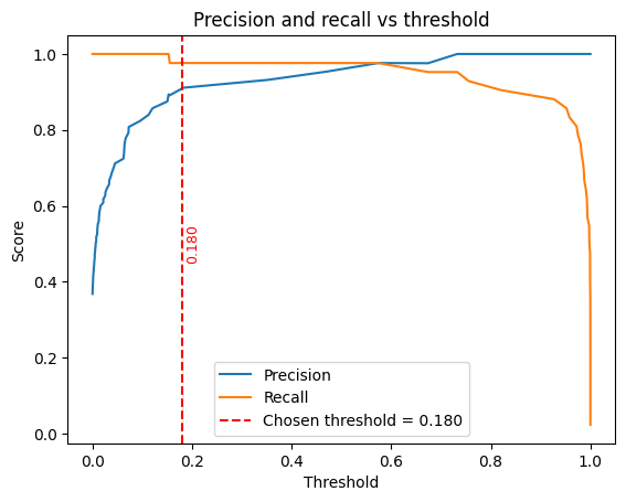
Model report:
    threshold            : 0.1802
    precision            : 0.9111
    recall               : 0.9762
    accuracy             : 0.9561
    confusion_matrix     :
[[68  4]
 [ 1 41]]
Conclusion
- The models show strong ability to distinguish between malignant and benign tumors.
- best_model achieved the highest performance, with 95.6% accuracy and 97.6% recall.
- This demonstrates the potential of ML in assisting medical diagnostics.
Note: This project is for educational and demonstration purposes only. It should not be used for clinical decision-making.
Next Steps
Potential improvements:
- Feature selection to reduce dimensionality
- Ensemble methods for better generalization
- Deployment as a simple web app (e.g., with Flask or Streamlit)
This would make the project even more practical and showcase end-to-end ML engineering skills.