%matplotlib inline
import numpy as np
np.set_printoptions(precision=3)
import pandas as pd
import matplotlib.pyplot as plt
import matplotlib.ticker as mtick
import seaborn as sns
import jsonCredit Risk Analysis
| Author: | Mahbub Alam |
Introduction
End-to-end Credit Risk Analysis using the German Credit dataset.
Steps:
- Data quality checks
- Exploratory data analysis (EDA)
- PD (Probability of Default) modeling and model validation (using Pipeline, GridSearchCV, and CalibratedClassifierCV)
- LGD (Loss Given Default) simulation + Random Forest model
- EAD (Exposure at Default) simulation
- ECL (Expected Credit Loss) calculation
- Visualization of risk segments, summaries by Purpose, Property, and EAD buckets
- Stress testing under adverse scenarios
Data quality checks
Summary:
- Inspect schema and datatypes
- Check for missing values
- Remove duplicates
- Count unique values per column
- Check class balance of the target (Risk: good/bad)
df = pd.read_csv('full_german_credit_dataset.csv')
# print(df.head())

print(f"")
print(df.info())

# Check missing data
missing_data = df.isna().any()
print(f"Missing data? - {'Yes' if missing_data.any() else 'No'}")

# Drop perfect duplicate rows
before = len(df)
df = df.drop_duplicates()
print(f"Duplicates removed: {before - len(df)}")

# check unique values
nunique = df.nunique().to_dict()
print(f"")
print(f"Unique values per column:\n\n{json.dumps(nunique, indent=4)}")

# Zero-variance check
zero_var = np.array([k for k in nunique if nunique[k] <= 1])
print(f"")
print(f"No. of columns with no variability (only one unique value): {len(zero_var)}")

print(f"")
# print(df['Risk'].head())
vc = df['Risk'].value_counts()
vcp = df['Risk'].value_counts(normalize=True)

class_balance = pd.DataFrame({'count' : vc, 'proportion' : vcp})

print(f"")
print(f"Class balance of the target (Risk):\n\n{class_balance}")
<class 'pandas.core.frame.DataFrame'>
RangeIndex: 1000 entries, 0 to 999
Data columns (total 21 columns):
 #   Column                                                    Non-Null Count  Dtype
---  ------                                                    --------------  -----
 0   Status_of_existing_checking_account                       1000 non-null   object
 1   Duration_in_month                                         1000 non-null   int64
 2   Credit_history                                            1000 non-null   object
 3   Purpose                                                   1000 non-null   object
 4   Credit_amount                                             1000 non-null   int64
 5   Savings_account_bonds                                     1000 non-null   object
 6   Present_employment_since                                  1000 non-null   object
 7   Installment_rate_in_percentage_of_disposable_income       1000 non-null   int64
 8   Personal_status_and_sex                                   1000 non-null   object
 9   Other_debtors_guarantors                                  1000 non-null   object
 10  Present_residence_since                                   1000 non-null   int64
 11  Property                                                  1000 non-null   object
 12  Age_in_years                                              1000 non-null   int64
 13  Other_installment_plans                                   1000 non-null   object
 14  Housing                                                   1000 non-null   object
 15  Number_of_existing_credits_at_this_bank                   1000 non-null   int64
 16  Job                                                       1000 non-null   object
 17  Number_of_people_being_liable_to_provide_maintenance_for  1000 non-null   int64
 18  Telephone                                                 1000 non-null   object
 19  Foreign_worker                                            1000 non-null   object
 20  Risk                                                      1000 non-null   object
dtypes: int64(7), object(14)
memory usage: 164.2+ KB
None
Missing data? - No
Duplicates removed: 0

Unique values per column:

{
    "Status_of_existing_checking_account": 4,
    "Duration_in_month": 33,
    "Credit_history": 5,
    "Purpose": 10,
    "Credit_amount": 921,
    "Savings_account_bonds": 5,
    "Present_employment_since": 5,
    "Installment_rate_in_percentage_of_disposable_income": 4,
    "Personal_status_and_sex": 4,
    "Other_debtors_guarantors": 3,
    "Present_residence_since": 4,
    "Property": 4,
    "Age_in_years": 53,
    "Other_installment_plans": 3,
    "Housing": 3,
    "Number_of_existing_credits_at_this_bank": 4,
    "Job": 4,
    "Number_of_people_being_liable_to_provide_maintenance_for": 2,
    "Telephone": 2,
    "Foreign_worker": 2,
    "Risk": 2
}

No. of columns with no variability (only one unique value): 0


Class balance of the target (Risk):

      count  proportion
Risk
good    700         0.7
bad     300         0.3
Encoding Risk
Encoding target variable Risk into numeric (1=bad, 0=good). This prepares the dataset for supervised learning models.
df["Risk"] = (df["Risk"] == "bad").astype(int)EDA with Account status, Loan amount and Age
Exploring how credit risk correlates with key features such as:
- Account status (barplot of default rates)
- Loan amount (boxplots by Risk)
- Age (histograms + median lines by Risk)
import textwrap

def wrap_labels_(ax, width=15, rotation=0, ha="right", pad=5):# {{{
    """Wrap long labels on x-axis"""
    ticks = ax.get_xticks()
    labels = [label.get_text() for label in ax.get_xticklabels()]

    # Wrap long labels
    wrapped_labels = ["\n".join(textwrap.wrap(l, width=width)) for l in labels]

    # Set ticks + labels explicitly
    ax.set_xticks(ticks)
    if ha == "at_tick":
        ax.set_xticklabels(wrapped_labels, rotation=rotation)
        for label in ax.get_xticklabels():
            label.set_x(label.get_position()[0])
    else:
        ax.set_xticklabels(wrapped_labels, rotation=rotation, ha=ha)

    # Adjust padding
    ax.tick_params(axis="x", pad=pad)


_, axes = plt.subplots(1, 3, figsize=(18, 6), num="risk_vs_acc_status_credit_amount_and_age")
# risk vs account status
ax = sns.barplot(
    x="Status_of_existing_checking_account",
    y="Risk",
    data=df,
    errorbar=None,
    estimator=np.mean,
    ax=axes[0]
)

# adding percentage on top of the bars
for p in ax.patches:
    value = p.get_height()
    ax.annotate(f"{value:.0%}",
                (p.get_x() + p.get_width()/2, value),
                ha="center", va="bottom", fontsize=10)

ax.yaxis.set_major_formatter(mtick.PercentFormatter(xmax=1, decimals=0))
wrap_labels_(ax, width=18, rotation=30, ha="at_tick", pad=10)
ax.set_title("Default Rate by Checking Account Status")
ax.set_ylabel("Default Rate")

# risk vs credit amount
ax = sns.boxplot(
    x="Risk",
    y="Credit_amount",
    data=df,
    # showfliers=False,
    hue="Risk",
    dodge=False,
    palette="Set2",
    ax=axes[1]
)

# Add median annotations
medians = df.groupby("Risk")["Credit_amount"].median()
for i, median in enumerate(medians):
    ax.text(i, median, f"{median:,.0f}",
            ha="center", va="bottom", fontsize=10, fontweight="bold", color="black")
ax.set_ylim(0, 10000)
ax.set_title("Loan Amount Distribution by Credit Risk")
ax.set_xlabel("Risk")
ax.set_ylabel("Credit Amount")

# risk vs age
ax = sns.histplot(
    data=df,
    x="Age_in_years",
    hue="Risk",
    bins=10,
    multiple="dodge",
    stat="percent",
    common_norm=False,
    palette="Set2",
    ax=axes[2]
)

# Add median lines for each group
medians = df.groupby("Risk")["Age_in_years"].median()
colors = {0: "green", 1: "red"}

for risk_val, median in medians.items():
    ax.axvline(median, color=colors[risk_val], linestyle="--", linewidth=1.5)
    ax.text(median, ax.get_ylim()[1]*0.9, f"Median {median:.0f}",
            rotation=90, ha="left", va="top", fontsize=10)

ax.set_title("Age Distribution by Credit Risk")
ax.set_xlabel("Age_in_years")
ax.set_ylabel("Share of Customers (%)")

for ax in axes:
    ax.xaxis.set_label_coords(0.5, -0.45)

plt.tight_layout(pad=1.5)
plt.subplots_adjust(wspace=0.25)
plt.savefig('risk_vs_acc_status_credit_amount_and_age.jpg')
plt.show()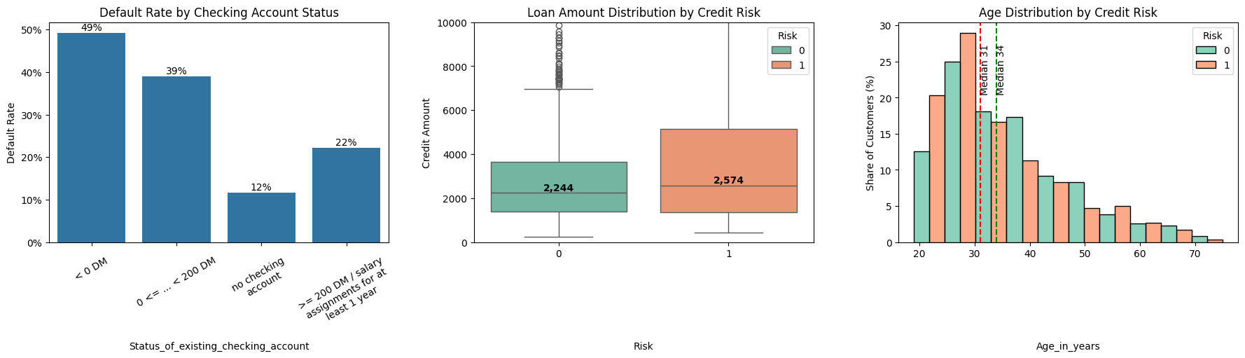
PD model
This is the Probability of Default (PD) modeling step (Basel/IFRS 9).
- Train Logistic Regression model to predict PD.
- Use preprocessing pipeline with scaling + one-hot encoding.
- Tune hyperparameters via GridSearchCV (refit on ROC-AUC).
- Calibrate final model using isotonic regression to align predicted PDs with observed default rates (CalibratedClassifierCV).
from sklearn.model_selection import train_test_split, GridSearchCV, StratifiedKFold
from sklearn.compose import ColumnTransformer
from sklearn.preprocessing import StandardScaler, OneHotEncoder
from sklearn.pipeline import Pipeline
from sklearn.linear_model import LogisticRegression
from sklearn.calibration import CalibratedClassifierCV
from sklearn.metrics import (roc_auc_score, brier_score_loss,
                             make_scorer, average_precision_score, roc_curve,
                             confusion_matrix, accuracy_score, recall_score)

X = df.drop(columns=['Risk']).copy()
y = df['Risk']

num_features = X.columns[X.dtypes.apply(lambda dt : np.issubdtype(dt, np.number))].tolist()
cat_features = [col for col in X.columns if col not in num_features]

X_train, X_test, y_train, y_test = train_test_split(X, y, test_size = 0.2, random_state = 42, stratify=y)

pre = ColumnTransformer(
    transformers = [
        ("num", StandardScaler(), num_features),
        ("cat", OneHotEncoder(), cat_features)
    ])

pd_pipe = Pipeline([
    ("pre", pre),
    ("logreg", LogisticRegression(max_iter = 1000, solver = "liblinear", random_state = 1))
])

hparams = {
    'logreg__penalty': ['l1', 'l2'],
    'logreg__C': np.logspace(-3, 3, 13),
    'logreg__class_weight': [None, 'balanced'],
    'logreg__fit_intercept': [True, False],
    'logreg__tol': [1e-4, 1e-5]
}

cv = StratifiedKFold(n_splits=5, shuffle=True, random_state = 2)

scorers = {
    "roc_auc": "roc_auc",
    "pr_auc": make_scorer(average_precision_score, response_method="predict_proba"),
    "brier": make_scorer(brier_score_loss, response_method="predict_proba", greater_is_better=False)
}

grid = GridSearchCV(
    pd_pipe,
    hparams,
    scoring = scorers,
    cv = cv,
    n_jobs = 4,
    refit = "roc_auc"
)

grid.fit(X_train, y_train)
best_model = grid.best_estimator_

# Calibrate best model using isotonic regression, this ensures PDs align with observed default rates
cal_pd = CalibratedClassifierCV(estimator = best_model, method = "isotonic", cv = 5)
cal_pd.fit(X_train, y_train)
CalibratedClassifierCV(cv=5,
estimator=Pipeline(steps=[('pre',
ColumnTransformer(transformers=[('num',
StandardScaler(),
['Duration_in_month',
'Credit_amount',
'Installment_rate_in_percentage_of_disposable_income',
'Present_residence_since',
'Age_in_years',
'Number_of_existing_credits_at_this_bank',
'Number_of_people_being_liable_to_provide_maintenance_for']...
'Purpose',
'Savings_account_bonds',
'Present_employment_since',
'Personal_status_and_sex',
'Other_debtors_guarantors',
'Property',
'Other_installment_plans',
'Housing',
'Job',
'Telephone',
'Foreign_worker'])])),
('logreg',
LogisticRegression(C=np.float64(0.03162277660168379),
fit_intercept=False,
max_iter=1000,
random_state=1,
solver='liblinear'))]),
method='isotonic')In a Jupyter environment, please rerun this cell to show the HTML representation or trust the notebook. On GitHub, the HTML representation is unable to render, please try loading this page with nbviewer.org.
Parameters
| estimator | Pipeline(step...liblinear'))]) | |
| method | 'isotonic' | |
| cv | 5 | |
| n_jobs | None | |
| ensemble | 'auto' |
Parameters
| transformers | [('num', ...), ('cat', ...)] | |
| remainder | 'drop' | |
| sparse_threshold | 0.3 | |
| n_jobs | None | |
| transformer_weights | None | |
| verbose | False | |
| verbose_feature_names_out | True | |
| force_int_remainder_cols | 'deprecated' |
['Duration_in_month', 'Credit_amount', 'Installment_rate_in_percentage_of_disposable_income', 'Present_residence_since', 'Age_in_years', 'Number_of_existing_credits_at_this_bank', 'Number_of_people_being_liable_to_provide_maintenance_for']
Parameters
| copy | True | |
| with_mean | True | |
| with_std | True |
['Status_of_existing_checking_account', 'Credit_history', 'Purpose', 'Savings_account_bonds', 'Present_employment_since', 'Personal_status_and_sex', 'Other_debtors_guarantors', 'Property', 'Other_installment_plans', 'Housing', 'Job', 'Telephone', 'Foreign_worker']
Parameters
| categories | 'auto' | |
| drop | None | |
| sparse_output | True | |
| dtype | <class 'numpy.float64'> | |
| handle_unknown | 'error' | |
| min_frequency | None | |
| max_categories | None | |
| feature_name_combiner | 'concat' |
Parameters
| penalty | 'l2' | |
| dual | False | |
| tol | 0.0001 | |
| C | np.float64(0....2277660168379) | |
| fit_intercept | False | |
| intercept_scaling | 1 | |
| class_weight | None | |
| random_state | 1 | |
| solver | 'liblinear' | |
| max_iter | 1000 | |
| multi_class | 'deprecated' | |
| verbose | 0 | |
| warm_start | False | |
| n_jobs | None | |
| l1_ratio | None |
Model validation
Generating validation report for the PD model. Discrimination (ROC-AUC, Gini) and calibration (Brier score) are the primary validation metrics.
- ROC-AUC and Gini coefficient (discrimination power)
- Brier score (calibration quality)
- Average precision score
- KS statistic (max separation between good/bad)
Threshold-based metrics at KS-optimal threshold:
- KS-optimal threshold
- Metrics at that threshold: Accuracy, Recall, Specificity, Confusion matrix
proba_test = cal_pd.predict_proba(X_test)[:,1]
print(f"Test AUC: {roc_auc_score(y_test, proba_test):.3f}")
gini = 2*roc_auc_score(y_test, proba_test) - 1
print(f"Gini coefficient: {gini:.3f}")
print(f"Brier score: {brier_score_loss(y_test, proba_test):.4f}")
print(f"Average precision score: {average_precision_score(y_test, proba_test):.4f}")

fpr, tpr, thresholds = roc_curve(y_test, proba_test)
ks_index = (tpr - fpr).argmax()
ks_stat = tpr[ks_index] - fpr[ks_index]
print(f"KS Statistic: {ks_stat:.3f}")

print(f"")
y_pred_ks = (proba_test >= thresholds[ks_index]).astype(int)
print(f"Optimal KS threshold: {thresholds[ks_index]:.3f}")
print("Diagnostic metrics at KS threshold:")
print(f"    Accuracy: {accuracy_score(y_test, y_pred_ks):.3f}")
print(f"    Recall: {recall_score(y_test, y_pred_ks):.3f}")

tn, fp, fn, tp = confusion_matrix(y_test, y_pred_ks).ravel()
specificity = tn / (tn + fp)
print(f"    Specificity (good capture rate): {specificity:.3f}")
print(f"    Confusion Matrix:\n {confusion_matrix(y_test, y_pred_ks)}")
Test AUC: 0.797
Gini coefficient: 0.593
Brier score: 0.1595
Average precision score: 0.6433
KS Statistic: 0.538
Optimal KS threshold: 0.363
Diagnostic metrics at KS threshold:
Accuracy: 0.770
Recall: 0.767
Specificity (good capture rate): 0.771
Confusion Matrix:
[[108 32]
[ 14 46]]Save the model for later
import joblib

joblib.dump(cal_pd, "pd_model_calibrated.pkl")

# Load model
# cal_pd = joblib.load("pd_model_calibrated.pkl")['pd_model_calibrated.pkl']LGD
The german credit dataset lacks information on recoveries for defaulted loans, so Loss Given Default (LGD) cannot be observed directly. We simulate LGD using a rule-based approach with random noise based on borrowers property, account status, savings, and purpose.
Later we will train a RandomForest model to estimate LGD from historical data (treating part our simulation as historical data). Predictions are floored at 10% in line with regulatory requirements CRR Article 164(4).
df_lgd = df.copy()

def lgd_simulation(row):
    # setting base lgd
    lgd = 0.55

    prop = row.get("Property").lower()
    check = row.get("Status_of_existing_checking_account").lower()
    savings = row.get("Savings_account_bonds").lower()
    purpose = row.get("Purpose").lower()

    # Collateral
    if "real estate" in prop or "building" in prop:
        lgd -= 0.20
    elif "car" in prop:
        lgd -= 0.10
    elif "unknown" in prop:
        lgd += 0.05

    # Liquidity buffers
    if ">= 200" in check:
        lgd -= 0.05
    if ">= 1000" in savings or "rich" in savings:
        lgd -= 0.05

    # Purposes that are typically less collateralized
    if purpose in ["education", "retraining", "others"]:
        lgd += 0.05

    return float(np.clip(lgd, 0.05, 0.95))

df_lgd["LGD_prior"] = df_lgd.apply(lgd_simulation, axis=1)

# Adding a randon noise to our simulation
rng = np.random.default_rng(42)
df_lgd["LGD_obs"] = np.where(
    df_lgd["Risk"] == 1,
    np.clip(df_lgd["LGD_prior"] + rng.normal(0, 0.01, size=len(df_lgd)), 0.01, 0.99),
    0.0
)
Simulate true defaulters
Summary:
- Sample 90% of bad credits as “true defaulters”, using PD-weighted probabilities.
- Assume that only those bad credits truly defaulted.
- Use this as “historical training data” for LGD modeling.
df_lgd["PD"] = cal_pd.predict_proba(X)[:,1]

bad_index = np.where(df_lgd["Risk"] == 1)[0]
weights = df_lgd.loc[bad_index, "PD"].to_numpy()
weights = weights / weights.sum()

rng = np.random.default_rng(43)
true_defaults = rng.choice(bad_index, size=int(0.9 * len(bad_index)), replace=False, p=weights)

df_lgd["true_default"] = 0
df_lgd.loc[true_defaults, "true_default"] = 1
Random forest model for LGD
Summary:
- Train Random Forest regressor on simulated LGD data.
- Predict expected LGD (LGD_exp) for entire portfolio.
- Expected LGD predictions are floored at 10% to align with CRR Article 164(4).
from sklearn.ensemble import RandomForestRegressor

X_lgd = df_lgd.loc[true_defaults].drop(columns=["Risk", "PD", "true_default", "LGD_prior", "LGD_obs"]).copy()
y_lgd = df_lgd.loc[true_defaults, "LGD_obs"]
# print(y_lgd.head())

lgd_pre = ColumnTransformer(
    transformers=[
        ("num", StandardScaler(), num_features),
        ("cat", OneHotEncoder(), cat_features),
    ]
)

lgd_model = Pipeline([
    ("pre", lgd_pre),
    ("rf", RandomForestRegressor(n_estimators=300, random_state=40))
])

lgd_model.fit(X_lgd, y_lgd)

df_lgd["LGD_exp"] = np.clip(
    lgd_model.predict(df_lgd.drop(columns=["Risk", "true_default", "LGD_prior", "LGD_obs"])),
    0.10, 0.99
)
Exposure at Default
Simulating EAD since the dataset lacks this column.
Formula (Basel/IFRS 9 style):
EAD = Balance + CCF * Undrawn

Balance = Amount withdrawn - Amount repaid

CCF = Credit Conversion Factor = Percentage defaulters withdraw just before defaulting
In practice, banks use observed balances and limits. Assumptions:
- Base utilization: random 50–95% of the credit amount
- Risk adjustment: riskier borrowers (high PD) repay less
- CCF fixed at 80% (typical Basel retail assumption)
rng = np.random.default_rng(50)

base_frac = np.clip(rng.normal(0.65, 0.1, size=len(df_lgd)), 0.3, 0.8)

risk_adj = df_lgd["PD"] * 0.2
balance_frac = np.clip(base_frac + risk_adj, 0.5, 0.95)

df_lgd["Withdrawn"] = df_lgd["Credit_amount"] * balance_frac
df_lgd["Undrawn"] = df_lgd["Credit_amount"] - df_lgd["Withdrawn"]

repay_frac = (1 - df_lgd["PD"]) * 0.8
df_lgd["Repaid"] = df_lgd["Withdrawn"] * repay_frac
df_lgd["Balance"] = df_lgd["Withdrawn"] - df_lgd["Repaid"]

CCF = 0.8

df_lgd["EAD"] = df_lgd["Balance"] + CCF * df_lgd["Undrawn"]
Expected Credit Loss
This block computes 12-month ECL.
- Formula:
ECL = PD * LGD * EAD * discount factorWe report portfolio-level stats and segment summaries:
- By Purpose
- By Property * EAD buckets (qcut)
# EIR, one year discount, assumed flat 5% for demonstration
annual_rate = 0.05
discount_factor = 1/(1+annual_rate)

df_lgd["ECL_12m"] = df_lgd["PD"] * df_lgd["LGD_exp"] * df_lgd["EAD"] * discount_factor

print(df_lgd.loc[true_defaults, ["Credit_amount", "PD", "LGD_exp", "EAD", "ECL_12m"]].head())

# Portfolio summaries
print("\n=== Portfolio summary ===")
print("Total EAD:", df_lgd["EAD"].sum().round(2))
print("Total 12m ECL:", df_lgd["ECL_12m"].sum().round(2))
print("Average PD:", df_lgd["PD"].mean().round(3))
print("Average LGD (expected):", df_lgd["LGD_exp"].mean().round(3))
print("ECL / EAD (portfolio charge):", (df_lgd["ECL_12m"].sum() / df_lgd["EAD"].sum()).round(4))

# segment views; purpose and ECL_12m
purpose_ecl = df_lgd.groupby("Purpose")["ECL_12m"].sum()
purpose_ead = df_lgd.groupby("Purpose")["EAD"].sum()
print("\n=== Segment summary (by Purpose) ===")
print(purpose_ecl)
print(f"")
print("ECL density by Purpose:", (purpose_ecl / purpose_ead).round(3))

# Segment views ('Property' and credit size bucket)
EAD_bins = pd.qcut(df_lgd["EAD"], q=4, duplicates="drop")

seg = (
    df_lgd.groupby(["Property", EAD_bins], observed=True).agg(
        n_accounts = ("PD", "size"),
        avg_PD = ("PD", lambda x : round(x.mean(), 3)),
        avg_LGD = ("LGD_exp", lambda x : round(x.mean(), 3)),
        total_EAD = ("EAD", lambda x : round(x.sum(), 2)),
        total_ECL_12m = ("ECL_12m", lambda x : round(x.sum(), 2))
    )
    .reset_index()
    .rename(columns={"EAD": "EAD_bucket"})
)

seg["EAD_bucket"] = seg["EAD_bucket"].apply(
    lambda interval: f"({round(interval.left)}, {round(interval.right)}]"
)
seg["ECL_density"] = (seg["total_ECL_12m"] / seg["total_EAD"]).round(4)

seg.to_csv('segment_view_risk.csv', index=False)

print("\n=== Segment summary (Property x EAD quartiles) ===")
print(seg.head(12))
Credit_amount PD LGD_exp EAD ECL_12m
652 2303 0.531489 0.359326 1521.195638 276.681021
37 2100 0.354955 0.293431 1101.943958 109.307133
11 4308 0.933333 0.352556 3963.541164 1242.105770
835 1082 0.654954 0.444322 809.159763 224.260676
602 1837 0.836684 0.658926 1590.620854 835.170420
=== Portfolio summary ===
Total EAD: 1947602.14
Total 12m ECL: 388994.37
Average PD: 0.304
Average LGD (expected): 0.42
ECL / EAD (portfolio charge): 0.1997
=== Segment summary (by Purpose) ===
Purpose
business 62107.415868
car (new) 89684.227220
car (used) 57442.869251
domestic appliances 2448.678718
education 30987.449345
furniture/equipment 60683.183727
others 29062.256335
radio/TV 48750.111199
repairs 7401.139585
retraining 427.036980
Name: ECL_12m, dtype: float64
ECL density by Purpose: Purpose
business 0.237
car (new) 0.206
car (used) 0.185
domestic appliances 0.226
education 0.300
furniture/equipment 0.182
others 0.374
radio/TV 0.130
repairs 0.208
retraining 0.079
dtype: float64
=== Segment summary (Property x EAD quartiles) ===
Property EAD_bucket \
0 building society savings agreement / life insu... (124, 691]
1 building society savings agreement / life insu... (691, 1213]
2 building society savings agreement / life insu... (1213, 2346]
3 building society savings agreement / life insu... (2346, 17164]
4 car or other, not in attribute 6 (124, 691]
5 car or other, not in attribute 6 (691, 1213]
6 car or other, not in attribute 6 (1213, 2346]
7 car or other, not in attribute 6 (2346, 17164]
8 real estate (124, 691]
9 real estate (691, 1213]
10 real estate (1213, 2346]
11 real estate (2346, 17164]
n_accounts avg_PD avg_LGD total_EAD total_ECL_12m ECL_density
0 67 0.195 0.353 32913.11 2112.27 0.0642
1 47 0.293 0.346 43376.35 4111.39 0.0948
2 64 0.325 0.347 110146.51 12189.55 0.1107
3 54 0.428 0.351 229074.82 37153.57 0.1622
4 52 0.197 0.450 25838.35 2193.87 0.0849
5 94 0.236 0.448 88733.38 8850.88 0.0997
6 88 0.316 0.448 147690.47 20193.41 0.1367
7 98 0.437 0.448 433000.47 91624.63 0.2116
8 114 0.154 0.343 54223.28 2698.26 0.0498
9 82 0.202 0.345 74198.31 4911.87 0.0662
10 64 0.259 0.349 103137.92 9135.28 0.0886
11 22 0.390 0.348 83004.16 11417.23 0.1376 Visualizing the predictions
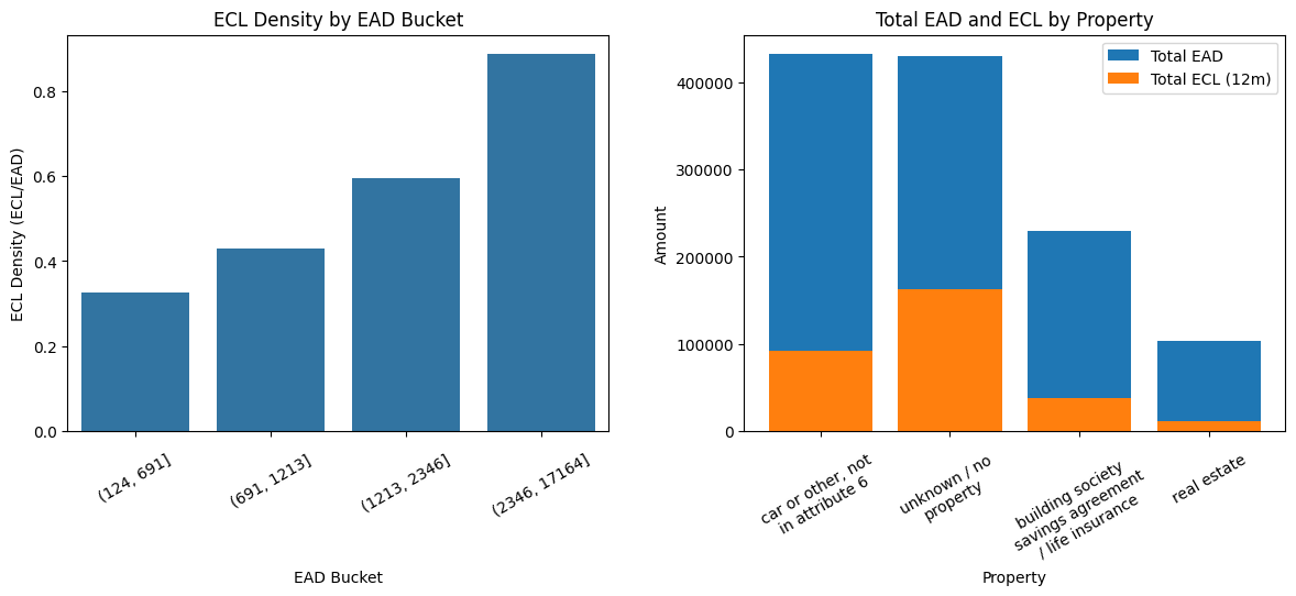
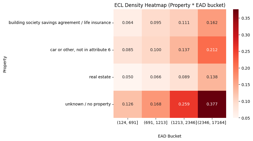
Visualize results with:
- ECL by Purpose (barplot)
- ECL density by EAD bucket
- Total EAD vs Total ECL by Property
- ECL density heatmap (Property * EAD bucket)
pur_summary = pd.DataFrame(
    purpose_ecl.sort_values(ascending=False).reset_index(),
    columns = np.array(["Purpose", "ECL_12m"])
)

plt.figure(num="ECL by Loan Purpose", figsize=(7,4))
sns.barplot(data=pur_summary, x="ECL_12m", y="Purpose", hue="Purpose", palette="Reds_r")
plt.xlabel("Total 12m ECL")
plt.ylabel("Purpose")
plt.title("ECL by Loan Purpose")
plt.tight_layout()
plt.savefig(f'ECL_by_Loan_Purpose.jpg')
plt.show()

_, axes = plt.subplots(1, 2, figsize=(12, 6), num="risk_vs_acc_status_credit_amount_and_age")
# ECL density by EAD bucket
ax = sns.barplot(
    data=seg,
    x="EAD_bucket",
    y="ECL_density",
    estimator=sum,
    errorbar=None,
    ax=axes[0]
)

wrap_labels_(ax, width=18, rotation=30, ha="at_tick", pad=10)
ax.set_title("ECL Density by EAD Bucket")
ax.set_ylabel("ECL Density (ECL/EAD)")
ax.set_xlabel("EAD Bucket")

# Stacked bar chart total EAD and total ECL by Property
prop_summary = seg.sort_values("total_EAD", ascending=False)

axes[1].bar(prop_summary["Property"], prop_summary["total_EAD"], label="Total EAD")
axes[1].bar(prop_summary["Property"], prop_summary["total_ECL_12m"], label="Total ECL (12m)")
axes[1].set_title("Total EAD and ECL by Property")
axes[1].set_ylabel("Amount")
axes[1].set_xlabel("Property")
wrap_labels_(axes[1], width=18, rotation=30, ha="at_tick", pad=10)
axes[1].legend()

for ax in axes:
    ax.xaxis.set_label_coords(0.5, -0.35)

plt.tight_layout(pad=1.5)
plt.subplots_adjust(wspace=0.25)
plt.savefig('ECL_density_total_EAD_EAD_bucket_Property.jpg')
plt.show()

# ECL density heatmap (Property * EAD bucket)
heatmap_data = seg.pivot_table(index="Property", columns="EAD_bucket",
                               values="ECL_density", aggfunc="mean", observed=True)

plt.figure(num="ECL Density Heatmap (Property * EAD bucket)", figsize=(9,5))
sns.heatmap(heatmap_data, annot=True, fmt=".3f", cmap="Reds")
plt.title("ECL Density Heatmap (Property * EAD bucket)")
plt.ylabel("Property")
plt.xlabel("EAD Bucket")
plt.gca().xaxis.set_label_coords(0.5, -0.15)
plt.tight_layout()
plt.savefig(f'ECL_density_heatmap.jpg')
plt.show()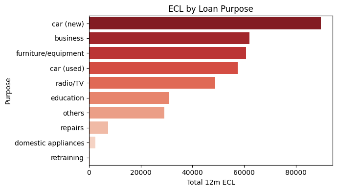
Stress testing predictions
Stress-test portfolio under adverse conditions:
- PD +50%
- LGD +20%
- Both combined
- Severe scenario (PD×2, LGD×1.5)
Reporting changes in portfolio ECL vs base case.
# already computed
base_ecl = df_lgd["ECL_12m"].sum().round(2)
print("Base case ECL (12m):", base_ecl)

# stress scenarios
stress_scenarios = {
    "PD +50%": {"PD": 1.5, "LGD": 1.0},
    "LGD +20%": {"PD": 1.0, "LGD": 1.2},
    "PD +50% & LGD +20%": {"PD": 1.5, "LGD": 1.2},
    "Severe stress (PD×2, LGD×1.5)": {"PD": 2.0, "LGD": 1.5}
}

# Apply scenarios
results = {}
for name, factors in stress_scenarios.items():
    df_stress = df_lgd.copy()
    df_stress["PD_stress"] = (df_stress["PD"] * factors["PD"]).clip(upper=1.0)
    df_stress["LGD_stress"] = (df_stress["LGD_exp"] * factors["LGD"]).clip(upper=1.0)
    df_stress["ECL_stress"] = (
        df_stress["PD_stress"] * df_stress["LGD_stress"] * df_stress["EAD"] * discount_factor
    )
    results[name] = df_stress["ECL_stress"].sum().round(2)

# results
print("\nStress Test Results")
for scenario, ecl in results.items():
    print(f"    {scenario:30} : {ecl}  (vs base {base_ecl}, change {((ecl/base_ecl)-1)*100:.1f}%)")
Base case ECL (12m): 388994.37
Stress Test Results
PD +50% : 538802.69 (vs base 388994.37, change 38.5%)
LGD +20% : 466793.24 (vs base 388994.37, change 20.0%)
PD +50% & LGD +20% : 646563.23 (vs base 388994.37, change 66.2%)
Severe stress (PD×2, LGD×1.5) : 927289.15 (vs base 388994.37, change 138.4%)